Browsing and analysing SalmoNet 2 data in Cytoscape
Prerequisites
> An up-to-date version of Cytoscape, available from: https://cytoscape.org/
Downloading data
> Download SalmoNet data from the website: http://salmonet.org/download
> Select the Strain, Layer, and output Format, and click on the Download button.
Importing data
> If you downloaded a .cys format network file, open it with File → Open ...
> If you downloaded a .cys or PSI-MITAB file, import it with the File → Import → Network from File option
>> After selecting the import option, you will be greeted by a window like the following:
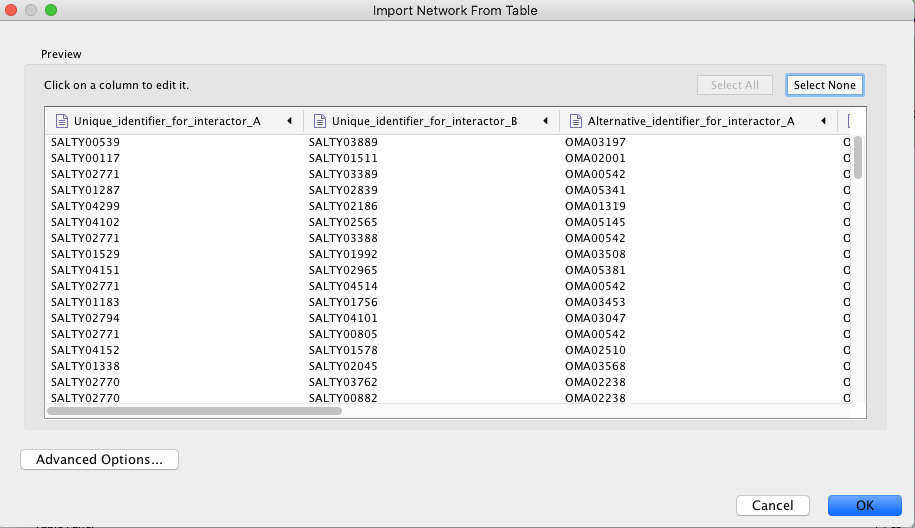
For a better resolution, please click on the image
>> The pictograms show the category you would like to place the individual columns into. The green and orange dot are the "main" source and target nodes, while the green and orange file icons will be your node attributes, like alternative IDs.
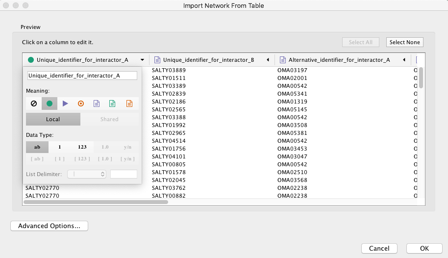
>> Make sure you select the green dot for the source interactor.
For a better resolution, please click on the image
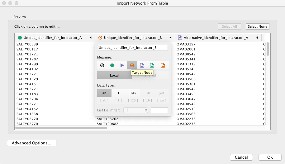
>> And select the orange circles for the target interactor.
For a better resolution, please click on the image
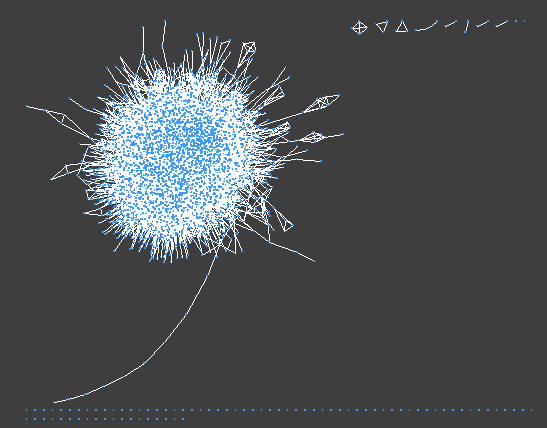
>> If everything goes well after a bried loadtime you should see a network like this:
For a better resolution, please click on the image
The Cytoscape GUI
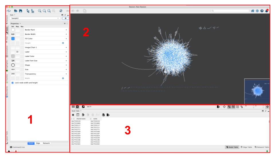
For a better resolution, please click on the image
The user interface has 3 main elements:
> 1: The panel on the left lets you select the visual mapping options (Node, Edge, and Network tabs on the bottom)
> 2: The main window visualizes the network and its layout, and lets you manipulate nodes/edges directly
> 3: The table pane on the bottom lets you look at the network data directly. Node table contains information pertaining to nodes, the Edge table to edges, and the Network table to the networks
Network analysis
Our networks only contain interaction and potential annotation data by default. To identify and visualize the inherent characteristics of our network, we will run a group of network analysis methods on them. Thankfully Cytoscape can calculate the most important metrics by default, and there are more methods available through the Cytoscape app store.
To run the network analysis, select the Tools menu point from the toolbar, and click on Network Analysis. After a few seconds a number of new columns should show up in the Node Table of our network.
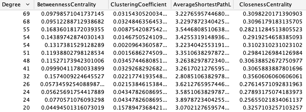
For a better resolution, please click on the image
These statistics can tell us a lot about the networks and nodes we are analysing. For example, the degree of a node notes the amount of neighbours it has in the network. These high degree nodes, also known as hubs, are often important biologically, taking part in many processes. To read more about the rest of the metrics we recommend the freely available online Barabasi (http://networksciencebook.com/).
Importing expression data
Download a subset of data from an applicable source. In this example we are using inter-strain relative expression levels from the SalComD23580 database. Select a group of genes, and download the resulting table. (http://bioinf.gen.tcd.ie/cgi-bin/salcom_v2.pl?_HL).
Download and load the S. Typhimurium 4/74 network from the SalmoNet website, and load it into Cytoscape using the steps outlined above.
To overlay the expression data open the downloaded expression table file:
> File → Import → Table from File ...
> Select the expression file from the file system
> Clicking on import will open a window like this:

For a better resolution, please click on the image
To match the network information with the expression information we need to find the matching identifiers to combine the data on. The Key Column for Network toggle lets you select the column to match on from the network's side, and clicking on the columns from the table below, and selecting the key icon lets you indicate the column to match on from the table's side.
After a brief load time the new columns will appear in the node table.
Visualizing expression data
To visualise the expression data in the context of the network, we need to select the rows we would like to analyse from the table, and their first neighbours so we add some context to the subset.
> This can be done by holding down the
> Click on
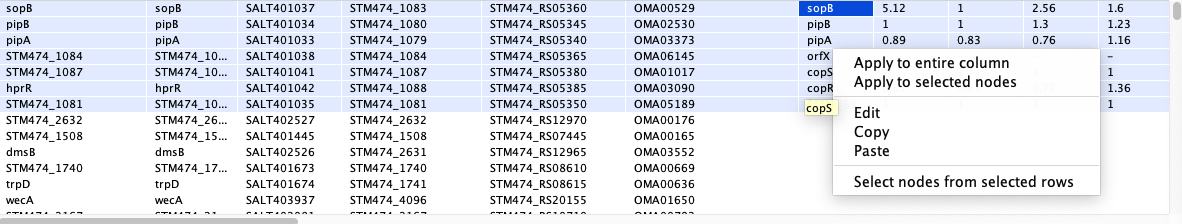
For a better resolution, please click on the image
> This will highlight the nodes in your network, and reduce the amount of hits in the table column to only the selected ones.
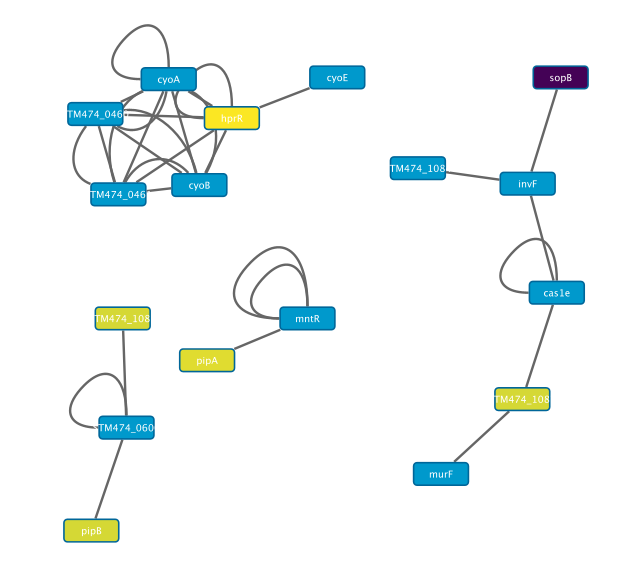
> To select their first neighbours use Select → Nodes → First Neighbours of Selected Nodes → Undirected
> Create a new subnetwork from your selection File → New Network → From Selected Nodes, All Edges

For a better resolution, please click on the image
> To visualize the expression differences select the Style panel on the side of the window.
>> Click on Fill color, select an environment (e.g. EEP), and select Continuous mapping from the second row

For a better resolution, please click on the image
>> This mapping function takes the values out of our data (i.e. the EEP column), and maps them to a visual value, in this case the node fill colour, visualizing the expression values of the impacted nodes.
For a better resolution, please click on the image
>> For nodes where no such data was imported, the default color remains, blue in this case.